文章目录
🚗 IV. Mothon Planning(运动规划)🟢 D. Graph Search Methods(图搜索算法)🟥 1) Lane Graph(车道图)🟧 2) Geometric Methods(几何方法)🟨 3) Sampling-based Methods(基于采样的方法)🟩 4) Graph Search Strategies( 图搜索策略)🔵 E. Incremental Search Techniques(增量搜索技术)🟣 F. Practical Deployments(实际部署)🚗 IV. Mothon Planning(运动规划)
🟢 D. Graph Search Methods(图搜索算法)
Although useful in many contexts, the applicability of variational methods is limited by their convergence to only local minima. In this section, we will discuss the class of methods that attempts to mitigate the problem by performing global search in the discretized version of the path space. These socalled graph search methods discretize the configuration space X\mathcal{X}X of the vehicle and represent it in the form of a graph and then search for a minimum cost path on such a graph.
尽管变分法在许多情况下都很有用,但是由于其仅收敛于局部最小值,其适用性因此受到限制。在本节中,我们将讨论一类方法。这些方法试图通过在路径空间的离散化版本中执行全局搜索来解决问题。这些所谓的图搜索方法离散化车辆的构型空间 X\mathcal{X}X ,并将其表示为图的形式,然后在这样的图上搜索一条最小成本路径。
In this approach, the configuration space is represented as a graph G=(V,E)G=(V, E)G=(V,E), where V⊂XV \subset \mathcal{X}V⊂X is a discrete set of selected configurations called vertices and E={(oi,di,σi)}E=\left\{\left(o_i, d_i, \sigma_i\right)\right\}E={(oi,di,σi)} is the set of edges, where oi∈Vo_i \in Voi∈V represents the origin of the edge, did_idi represents the destination of the edge and σi represents the path segments connecting oi and did_idi. It is assumed that the path segment σi connects the two vertices: sigmai(0)=oisigma_i(0)=o_isigmai(0)=oi and sigmai(1)=disigma_i(1)=d_isigmai(1)=di。Further, it is assumed that the initial configuration xinit\mathrm{x}_{\text {init }}xinit is a vertex of the graph. The edges are constructed in such a way that the path segments associated with them lie completely in Xfree\mathcal{X}_{\text {free }}Xfree and satisfy differential constraints. As a result, any path on the graph can be converted to a feasible path for the vehicle by concatenating the path segments associated with edges of the path through the graph.
该方法中,构型空间表示为图 G=(V,E)G=(V, E)G=(V,E) ,其中V⊂XV \subset \mathcal{X}V⊂X 是所选构型的离散集合,称为顶点, E={(oi,di,σi)}E=\left\{\left(o_i, d_i, \sigma_i\right)\right\}E={(oi,di,σi)} 是边的集合,其中 oi∈Vo_i \in Voi∈V 表示边的原点/起点, did_idi 表示边的目的地/终点。sigmaisigma_isigmai表示连接 oio_ioi 和 did_idi 的路径段。我们假设路径段 $o_i $ 连接两个顶点 sigmai(0)=oisigma_i(0)=o_isigmai(0)=oi 和 sigmai(1)=disigma_i(1)=d_isigmai(1)=di 。此外,我们假设初始构型xinit\mathrm{x}_{\text {init }}xinit是图的一个顶点。边的构造满足以下条件:与边相对应的路径段完全处于 Xfree\mathcal{X}_{\text {free }}Xfree中,并且满足微分约束。如此一来,对于穿过图的路径,通过将该路径上的边所对应的路径段串联起来,便可以将图上的任何路径转换为车辆的一条可行路径。
There is a number of strategies for constructing a graph discretizing the free configuration space of a vehicle. In the following subsections, we discuss three common strategies: Hand-crafted lane graphs, graphs derived from geometric representations and graphs constructed by either control or configuration sampling.
目前存在许多策略可用于构造一个离散化车辆的自由构型空间的图。在以下的小节中,我们将讨论三种常见的策略:手工绘制的车道图,从几何表示中推导而得的图,以及通过控制或构型采样而构造的图。
1) Lane Graph: When the path planning problem involves driving on a structured road network, a sufficient graph discretization may consist of edges representing the path that the car should follow within each lane and paths that traverse intersections. Road lane graphs are often partly algorithmically generated from higher-level street network maps and partly human edited. An example of such a graph is in Figure IV.1.
🟥 1) Lane Graph(车道图)
当路径规划问题涉及在结构化的道路网络上行驶时,充分的图离散化可以由表示汽车在每条车道内应当遵循的路径和表示穿过交叉口的路径的边组成。道路车道图通常部分由较高级别的街道网络地图依靠算法生成,部分由人工编辑而得。图IV.1是这样的图的一个示例。
图 IV.1: 手工绘制图表示正常情况下的期望行驶路径。.
Although most of the time it is sufficient for the autonomous vehicle to follow the paths encoded in the road lane graph, occasionally it must be able to navigate around obstacles that were not considered when the road network graph was designed or in environments not covered by the graph. Consider for example a faulty vehicle blocking the lane that the vehicle plans to traverse – in such a situation a more general motion planning approach must be used to find a collision-free path around the detected obstacle.
尽管大多数时候让自动驾驶汽车沿着道路车道图中编码的路径行驶就足够了,但是有时它必须能在设计道路网络图时未考虑的障碍物周围导航,或者能在图中未涵盖的环境中导航。例如,考虑一辆故障车辆阻塞了我们的车辆计划穿过的车道,在这种情况下,必须使用更一般的运动规划方法,以找到被检测到的障碍物周围的一条无碰撞路径。
The general path planning approaches can be broadly divided into two categories based on how they represent the obstacles in the environment. So-called geometric or combinatorial methods work with geometric representations of the obstacles, where in practice the obstacles are most commonly described using polygons or polyhedra. On the other hand, socalled sampling-based methods abstract away from how the obstacles are internally represented and only assumes access to a function that determines if any given path segment is in collision with any of the obstacles.
根据环境中障碍物的表示方法,可以将一般的路径规划方法大致分为两类。所谓的几何或组合方法适用于障碍物的几何表示——在实践中,障碍物最常用多边形或多面体来描述。另一方面,所谓的基于采样的方法抽象了障碍物的内部表示方式,并且仅假设对于一个函数的访问,该函数用于确定任何给定的路径段是否与任何障碍物发生了碰撞。
2) Geometric Methods: In this section, we will focus on path planning methods that work with geometric representations of obstacles. We will first concentrate on path planning without differential constraints because for this formulation, efficient exact path planning algorithms exist. Although not being able to enforce differential constraints is limiting for path planning for traditionally-steered cars because the constraint on minimum turn radius cannot be accounted for, these methods can be useful for obtaining the lower- and upper- bounds on the length of a curvature-constrained path and for path planning for more exotic car constructions that can turn on the spot.
🟧 2) Geometric Methods(几何方法)
在本节中,我们将重点介绍使用障碍物几何表示的路径规划方法。我们将首先关注无微分约束的路径规划,因为对于此情况,存在有效的精确路径规划算法。尽管由于无法考虑对最小转弯半径的约束,因此无法强制地施加微分约束,进而对传统转向车辆的路径规划产生了限制,但是这些方法可用于求解具有曲率约束的路径的长度下限和上限[1],并且还可用于能够原地转弯的、更特殊的车辆结构的路径规划。
In path planning, the term roadmap is used to describe a graph discretization of Xfree\mathcal{X}_{\text {free }}Xfree that describes well the connectivity of the free configuration space and has the property that any point in Xfree\mathcal{X}_{\text {free }}Xfree is trivially reachable from some vertices of the roadmap. When the set Xfree can be described geometrically using a linear or semi-algebraic model, different types of roadmaps for Xfree\mathcal{X}_{\text {free }}Xfree can be algorithmically constructed and subsequently used to obtain complete path planning algorithms. Most notably, for Xfree⊂R2\mathcal{X}_{\text {free }} \subset \mathbb{R}^2Xfree⊂R2 and polygonal models of the configuration space, several efficient algorithms for constructing such roadmaps exists such as the vertical cell decomposition [93], generalized Voronoi diagrams [94], [95], and visibility graphs [33], [96]. For higher dimensional configuration spaces described by a general semi-algebraic model, the technique known as cylindrical algebraic decomposition can be used to construct a roadmap in the configuration space [47], [97] leading to complete algorithms for a very general class of path planning problems. The fastest of this class is an algorithm developed by Canny [65] that has (single) exponential time complexity in the dimension of the configuration space. The result is however mostly of a theoretical nature without any known implementation to date.
在路径规划中,术语路线图用于描述 Xfree\mathcal{X}_{\text {free }}Xfree的图离散化。这种离散化能够很好地描述自由构型空间的连通性,并且 Xfree\mathcal{X}_{\text {free }}Xfree中的任意点都可以从路线图的某些顶点出发而轻松到达。当集合 Xfree\mathcal{X}_{\text {free }}Xfree可以通过线性或半代数模型被几何形式地描述时,我们能在算法上构造用于 Xfree\mathcal{X}_{\text {free }}Xfree的不同类型的路线图,进而将其用于获得完备的路径规划算法。最值得注意的是,对于 Xfree⊂R2\mathcal{X}_{\text {free }} \subset \mathbb{R}^2Xfree⊂R2 和构型空间的多边形模型,存在几种用于构造这种路线图的有效算法,如垂直单元分解(vertical cell decomposition)[93]、广义冯洛诺伊图(generalized Voronoi diagrams)[94][95]和可见图[33][96]。对于由一般半代数模型描述的高维构型空间,一种称为柱形代数分解(cylindrical algebraic decomposition)的技术可用于在构型空间中构造路线图[47][97],从而为非常一般的路径规划问题提供完备的算法。这类算法中最快的是Canny开发的算法[65],其在构型空间的维度上具有(单个)指数时间的复杂度。然而,其结论主要是理论性质的,迄今为止没有任何已知的实现。
Due to its relevance to path planning for car-like vehicles, a number of results also exist for the problem of path planning with a constraint on maximum curvature. Backer and Kirkpatrick [98] provide an algorithm for constructing a path with bounded curvature that is polynomial in the number of features of the domain, the precision of the input and the number of segments on the simplest obstacle-free Dubins path connecting the specified configurations. Since the problem of finding a shortest path with bounded curvature amidst polygonal obstacles is NP-hard, it is not surprising that no exact polynomial solution algorithm is known. An approximation algorithm for finding shortest curvature-bounded path amidst polygonal obstacles has been first proposed by Jacobs and Canny [99] and later improved by Wang and Agarwal [100] with time complexity O(n2ϵ4logn)O\left(\frac{n^2}{\epsilon^4} \log n\right)O(ϵ4n2logn), where n is the number of vertices of the obstacles and ϵ\epsilonϵ is the approximation factor. For the special case of so-called moderate obstacles that are characterized by smooth boundary with curvature bounded by κκκ, an exact polynomial algorithm for finding a path with curvature bounded by at most κκκ have been developed by Boissonnat and Lazard [73].
对于具有最大曲率约束的运动规划问题,目前也存在一些研究成果,这是因为该问题与类车车辆的运动规划存在关联。Backer和Kirkpatrick提出了一种算法[98],用于构造一条具有有界曲率的多项式路径,且该多项式是相对于以下变量而言的:域的特征的数量、输入的精度、连接特定构型的最简单的无障碍Dubins路径上的路径段个数。由于在多边形障碍物中找到一条具有有界曲率的最短路径的问题是NP困难的,因此目前并不存在精确的多项式解算法。Jacobs和Canny首先提出了一种在多边形障碍物中寻找曲率有界的最短路径的近似算法[99],后来Wang和Agarwal进行了改进[100],改进后的算法的时间复杂度为 O(n2ϵ4logn)O\left(\frac{n^2}{\epsilon^4} \log n\right)O(ϵ4n2logn) ,其中 n 是障碍物的顶点数, ϵ\epsilonϵ 是近似因子。所谓的中等障碍物(moderate obstacles)具有光滑的边界,且边界的曲率大小以 kkk 为界。在这种中等障碍物的特殊情况下,Boissonnat和Lazard开发了一种精确的多项式算法,以找到曲率最大以 kkk 为界的一条路径[73]。
3) Sampling-based Methods: In autonomous driving, a geometric model of Xfree\mathcal{X}_{\text {free }}Xfree is usually not directly available and it would be too costly to construct from raw sensoric data. Moreover, the requirements on the resulting path are often far more complicated than a simple maximum curvature constraint. This may explain the popularity of sampling-based techniques that do not enforce a specific representation of the free configuration set and dynamic constraints. Instead of reasoning over a geometric representation, the sampling based methods explore the reachability of the free configuration space using steering and collision checking routines:
🟨 3) Sampling-based Methods(基于采样的方法)
在自动驾驶中, Xfree\mathcal{X}_{\text {free }}Xfree 的几何模型通常不是直接可用的,而通过原始传感数据构造模型的成本又太高。此外,对生成路径的要求通常比简单的最大曲率约束更复杂。这可以解释基于采样的方法的流行,因为后者并未强制对自由构型集和动力学约束采用特定的表示方法。基于采样的方法不是通过几何表示进行推理,而是使用转向/引导(steering)和碰撞检测(collision checking)的推理方式来探索自由构型空间的可达性:
The steering function steer(x,y)\text { steer }(\mathrm{x}, \mathrm{y})steer(x,y) returns a path segment starting from configuration x\mathrm{x}x going towards configuration y\mathrm{y}y (but not necessarily reaching y\mathrm{y}y) ensuring the differential constraints are satisfied, i.e., the resulting motion is feasible for the vehicle model in consideration. The exact manner in which the steering function is implemented depends on the context in which it is used. Some typical choices encountered in the literature are:
转向/引导函数 steer(x,y)\text { steer }(\mathrm{x}, \mathrm{y})steer(x,y) 返回一条从构型 x\mathrm{x}x 出发、朝向构型 y\mathrm{y}y(但是不必须要到达 y\mathrm{y}y)的路径段,并确保满足微分约束,即生成的运动对于所考虑的车辆模型是可行的。转向函数的具体实现方式取决于其所处的环境。文献中报告过的一些典型选择包括:
1) Random steering: The function returns a path that results from applying a random control input through a forward model of the vehicle from state x\mathrm{x}x for either a fixed or variable time step [101].
2) Heuristic steering: The function returns a path that results from applying control that is heuristically constructed to guide the system from x\mathrm{x}x towards y\mathrm{y}y [102]–[104]. This includes selecting the maneuver from a predesigned discrete set (library) of maneuvers.
3) Exact steering: The function returns a feasible path that guides the system from x\mathrm{x}x to y\mathrm{y}y. Such a path corresponds to a solution of a 2-point boundary value problem. For some systems and cost functionals, such a path can be obtained analytically, e.g., a straight line for holonomic systems, a Dubins curve for forward-moving unicycle [57], or a Reeds-Shepp curve for bi-directional unicycle [58]. An analytic solution also exists for differentially flat systems [61], while for more complicated models, the exact steering can be obtained by solving the twopoint boundary value problem.
4) Optimal exact steering: The function returns an optimal exact steering path with respect to the given cost functional. In fact, the straight line, the Dubins curve, and the Reeds-Shepp curve from the previous point are optimal solutions assuming that the cost functional is the arc-length of the path [57], [58]
1) 随机转向:转向函数返回的路径是在状态x\mathrm{x}x时,将一个随机控制输入应用到车辆的前向模型、并经过一个固定或可变时间步长而得到的[101]。 2) 启发式转向:转向函数返回的路径是应用一个启发式构造的控制而得到的,这类启发式的构造方法用于引导系统从 x\mathrm{x}x 朝向 y\mathrm{y}y [102-104],包括从预先设计的离散策略集合(库)中选择一个策略。 3) 精确转向:转向函数返回一条用于引导系统从 x\mathrm{x}x 到 y\mathrm{y}y 的可行路径。这样一条路径对应一个两点边值问题的一个解。对于一些系统和成本泛函,可以解析地求出这样的路径,例如完整系统的一条直线、前向移动的单轮车的一条Dubins曲线[57]、或双向单轮车[58]的一条Reeds-Shepp曲线。微分平坦系统同样存在解析解[61],而对于更复杂的模型,可以通过求解两点边值问题来获得精确的转向解。 4) 最优精确转向:转向函数返回相对于给定的成本泛函的一条最优精确转向路径。事实上,若假设成本泛函是路径的弧长[57][58],则上一段提到的直线、Dubins曲线和Reeds-Shepp曲线都是最优解。
The collision checking function col-free(σ\sigmaσ) returns true if path segment σ\sigmaσ lies entirely in Xfree\mathcal{X}_{\text {free }}Xfree and it is used to ensure that the resulting path does not collide with any of the obstacles.
如果路径段 σ\sigmaσ 完全处于 Xfree\mathcal{X}_{\text {free }}Xfree中,那么碰撞检测函数 col-free(σ)\operatorname{col} \text {-free }(\sigma)col-free(σ) 将返回真值(即true),用于确保生成的路径不会与任何障碍物发生碰撞。
Having access to steering and collision checking functions, the major challenge becomes how to construct a discretization that approximates well the connectivity of Xfree\mathcal{X}_{\text {free }}Xfree without having access to an explicit model of its geometry. We will now review sampling-based discretization strategies from literature.
具备了转向函数和碰撞检测函数之后,主要的挑战就是如何构造一个能很好地近似 Xfree\mathcal{X}_{\text {free }}Xfree的连接性的离散化,而不需要拥有其几何结构的显式模型。接下来我们将从文献中回顾基于采样的离散化策略。
A straightforward approach is to choose a set of motion primitives (fixed maneuvers) and generate the search graph by recursively applying them starting from the vehicle’s initial configuration xinit\mathrm{x}_{\text {init}}xinit, e.g., using the method in Algorithm 1.
For path planning without differential constraints, the motion primitives can be simply a set of straight lines with different directions and lengths. For a car-like vehicle, such motion primitive might by a set of arcs representing the path the car would follow with different values of steering. A variety of techniques can be used for generating motion primitives for driverless vehicles. A simple approach is to sample a number of control inputs and to simulate forwards in time using a vehicle model to obtain feasible motions. In the interest of having continuous curvature paths, clothoid segments are also sometimes used [105]. The motion primitives can be also obtained by recording the motion of a vehicle driven by an expert driver [106].
一种直接的方法是选择一组运动基元(固定策略),然后从车辆的初始构型 xinit\mathrm{x}_{\text {init}}xinit出发,递归地应用这些基元,来生成搜索图,例如使用算法1的方法。对于没有微分约束的路径规划,运动基元可以简单地是一组具有不同方向和长度的直线。对于类车车辆,运动基元可以是一组弧,表示汽车以不同的转向值跟随的路径。多种技术都可用于生成无人驾驶车辆的运动基元。一种简单的方法是采样多个控制输入,并使用车辆模型实时模拟前进,以获得可行的运动。为了获得具有连续曲率的路径,有时也使用回旋曲线段[105]。此外,还可以通过记录由专家驾驶员驾驶的车辆的运动来获得运动基元[106]。
Observe that the recursive application of motion primitives may generate a tree graph in which in the worst-case no two edges lead to the same configuration. There are, however, sets of motion primitives, referred to as lattice-generating, that result in regular graphs resembling a lattice. See Figure IV.2a for an illustration. The advantage of lattice generating primitives is that the vertices of the search graph cover the configuration space uniformly, while trees in general may have a high density of vertices around the root vertex. Pivtoraiko et al. use the term “state lattice” to describe such graphs in [107] and point out that a set of lattice-generating motion primitives for a system in hand can be obtained by first generating regularly spaced configurations around origin and then connecting the origin to such configurations by a path that represents the solution to the two-point boundary value problem between the two configurations.
我们可以观察到,递归地应用运动基元能生成树图,这种图在最坏情况下,不存在两条能到达相同构型的边。然而,称为“栅格生成”的运动基元集能生成形似栅格的规则图形。见图4.2a,栅格生成基元的优点是搜索图的顶点能够均匀地覆盖构型空间,而树通常可能在根顶点的周围出现高密度分布的顶点。Pivtoraiko等人使用术语“状态栅格”来描述[107]中的此类图,并指出,如果首先在原点周围生成规则间隔的构型,然后通过表示两点边值问题的解的路径将原点连接到这种构型,就可以得到当前系统的一组栅格生成运动基元。
An effect that is similar to recursive application of latticegenerating motion primitives from the initial configuration can be achieved by generating a discrete set of samples covering the (free) configuration space and connecting them by feasible path segments obtained using an exact steering procedure.
通过生成覆盖(自由)构型空间的离散样本集,并通过使用精确的转向程序获得的可行路径段将它们连接起来,可以实现类似于从初始构型出发、递归地应用栅格生成运动基元的所产生的效果。
Most sampling-based roadmap construction approaches follow the algorithmic scheme shown in Algorithm 2, but differ in the implementation of the sample-points(X,n)\text { sample-points }(\mathcal{X}, n)sample-points(X,n) and neighbors(x,V)\text { neighbors }(\mathrm{x}, V)neighbors(x,V) routines. The function sample-points(X,n)\text { sample-points }(\mathcal{X}, n)sample-points(X,n) represents the strategy for selecting n points from the configuration space X\mathcal{X}X, while the function neighbors(x,V)\text { neighbors }(\mathrm{x}, V)neighbors(x,V) represents the strategy for selecting a set of neighboring vertices N⊆VN \subseteq VN⊆V for a vertex x, which the algorithm will attempt to connect to x by a path segment using an exact steering function, steerexact(x,y)\text { steer }_{\text {exact }}(\mathrm{x}, \mathrm{y})steerexact(x,y).
大多数基于采样的路线图的构造方法都遵循算法2所示的方案,但是在采样点函数 sample-points(X,n)\text { sample-points }(\mathcal{X}, n)sample-points(X,n) 和邻点函数 neighbors(x,V)\text { neighbors }(\mathrm{x}, V)neighbors(x,V) 的实现上有所不同。采样点函数 sample-points(X,n)\text { sample-points }(\mathcal{X}, n)sample-points(X,n)表示从构型空间 X\mathcal{X}X 中选择 n 个点的策略,而邻点函数neighbors(x,V)\text { neighbors }(\mathrm{x}, V)neighbors(x,V)表示为顶点 x 选择一组邻顶点 N⊆VN \subseteq VN⊆V 的策略。对于邻顶点 y,该算法将尝试通过精确转向函数 steerexact(x,y)\text { steer }_{\text {exact }}(\mathrm{x}, \mathrm{y})steerexact(x,y) 来找到一条从 y 连接到 x 的路径段。
The two most common implementations of neighbors(x,V)\text { neighbors }(\mathrm{x}, V)neighbors(x,V) function are 1) return n points arranged in a regular grid and 2) return n randomly sampled points from X\mathcal{X}X. While random sampling has an advantage of being generally applicable and easy to implement, so-called Sukharev grids have been shown to achieve optimal L1-dispersion in unit hypercubes, i.e. they minimize the radius of the largest empty ball with no sample point inside. For in depth discussion of relative merits of random and deterministic sampling in the context of sampling-based path planning, we refer the reader to [108]. The two most commonly used strategies for implementing neighbors(x,V)\text { neighbors }(\mathrm{x}, V)neighbors(x,V) function are to take 1) the set of k-nearest neighbors to x or 2) the set of points lying within the ball centered at x with radius rrr.
函数 sample-points(X,n)\text { sample-points }(\mathcal{X}, n)sample-points(X,n) 的最常见的两种实现方式是:(1)返回排列在一个规则网格中的 n 个点,(2)返回 X\mathcal{X}X 中的 n 个随机采样点。尽管随机抽样具有普遍适用和易于实施的优点,但所谓的Sukharev网格已经被证明在单位超立方体中实现了最优 L∞L_{\infty}L∞ 散度,即其最小化了内部没有采样点的最大空球的半径。为了深入讨论基于采样的路径规划环境中随机采样和确定性采样的相对优点,我们请读者参考[108]。实现函数 neighbors(x,V)\text { neighbors }(\mathrm{x}, V)neighbors(x,V) 的两个最常用策略是:(1)与 x 最近的 k 近邻的集合,(2)位于以 x 为中心的、半径为 rrr 的球内的点的集合。
In particular, samples arranged deterministically in a ddd-dimensional grid with the neighborhood taken as 4 or 8 nearest neighbors in 2-D or the analogous pattern in higher dimensions represents a straightforward deterministic discretization of the free configuration space. This is in part because they arise naturally from widely used bitmap representations of free and occupied regions of robots’ configuration space [109].
特别地,在ddd维网格中以确定性方式排列的样本,若其邻域在二维中取为 4 个或 8个最近邻、在更高维度中取为与二维情况相类似的模式,那么这些样本代表了自由构型空间的简单确定性离散化,部分是因为它们自然产生于机器人构型空间的自由和占用区域所广泛使用的位图表示[109]。
Kavraki et al. [110] advocate the use of random sampling within the framework of Probabilistic Roadmaps (PRM) in order to construct roadmaps in high-dimensional configuration spaces, because unlike grids, they can be naturally run in an anytime fashion. The batch version of PRM [79] follows the scheme in Algorithm 2 with random sampling and neighbors selected within a ball with fixed radius rrr. Due to the general formulation of PRMs, they have been used for path planning for a variety of systems, including systems with differential
constraints. However, the theoretical analyses of the algorithm have primarily been focused on the performance of the algorithm for systems without differential constraints, i.e. when a straight line is used to connect two configurations. Under such an assumption, PRMs have been shown in [80] to be probabilistically complete and asymptotically optimal. That is, the probability that the resulting graph contains a valid solution (if it exists) converges to one with increasing size of the graph and the cost of the shortest path in the graph converges to the optimal cost. Karaman and Frazzoli [80] proposed an adaptation of batch PRM, called PRM*, that instead only connects
neighboring vertices in a ball with a logarithmically shrinking radius with increasing number of samples to maintain both asymptotic optimality and computational efficiency.
Kavraki等人[110]主张在概率路线图框架内使用随机抽样,以便在高维构型空间中构造路线图,因为与网格不同,它们随时可以自然运行。批处理版本的PRM遵循算法2的方案,其采用随机抽样,并且在固定半径 rrr 的球内选择邻点[79]。由于PRM具有通用的形式,它们已用于各种系统的路径规划,包括具有微分约束的系统。然而,该算法的理论分析主要集中于无微分约束系统的算法性能,即,当使用直线连接两种构型时。在这样的假设下,文章[80]中的PRM被证明是概率完备且渐近最优的。也就是说,其生成的图包含有效解(如果存在)的概率随着图的大小的增加而收敛到 1,且图中最短路径的成本随之收敛到最优成本。Karaman和Frazzoli提出了一种称为PRM*的批处理PRM的自适应版本[80],其仅连接一个球内的邻顶点。该球的半径随着样本数量的增加而对数大小地减小。这么做的目的是保持算法的渐近最优性以及计算效率。
In the same paper, the authors propose Rapidly-exploring Random Graphs (RRG*), which is an incremental discretization strategy that can be terminated at any time while maintaining the asymptotic optimality property. Recently, Fast Marching Tree (FMT*) [111] has been proposed as an asymptotically optimal alternative to PRM*. The algorithm combines discretization and search into one process by performing a lazy dynamic programming recursion over a set of sampled vertices that can be subsequently used to quickly determine the path from initial configuration to the goal region.
在同一篇论文中,作者同时提出了快速探索随机图。这是一种增量离散化策略,在保持渐近最优性的同时能够随时终止。最近,快速行进树[111]被提出作为PRM*的渐近最优替代方案。该算法通过对一组采样顶点执行惰性动态规划递归,将离散化和搜索结合到一个过程中。这些采样顶点随后可以被用于快速确定从初始构型到目标区域的路径。
Recently, the theoretical analysis has been extended also to differentially constrained systems. Schmerling et al. [81] propose differential versions of PRM* and FMT* and prove asymptotic optimality of the algorithms for driftless controlaffine dynamical systems, a class that includes models of nonslipping wheeled vehicles.
最近,理论分析也扩展到微分约束系统。Schmerling等人[81]提出了PRM和FMT的微分版本,并证明了这些算法对于无漂移的仿射控制的动力系统的渐近最优性。这一类动力系统包括无滑移的轮式车辆模型。
4) Graph Search Strategies: In the previous section, we have discussed techniques for the discretization of the free configuration space in the form of a graph. To obtain an actual optimal path in such a discretization, one must employ one of the graph search algorithms. In this section, we are going to review the graph search algorithms that are relevant for path planning.
在上一节中,我们讨论了将自由构型空间离散化为图的形式的技术。为了在这种离散化中获得一条实际的最优路径,必须使用图搜索算法。在本节中,我们将回顾与路径规划相关的图搜索算法。
🟩 4) Graph Search Strategies( 图搜索策略)
The most widely recognized algorithm for finding shortest paths in a graph is probably the Dijkstra’s algorithm [32]. The algorithm performs the best first search to build a tree representing shortest paths from a given source vertex to all other vertices in the graph. When only a path to a single vertex is required, a heuristic can be used to guide the search process. The most prominent heuristic search algorithm is A* developed by Hart, Nilsson and Raphael [112]. If the provided15 heuristic function is admissible (i.e., it never overestimates the cost-to-go), A* has been shown to be optimally efficient and is guaranteed to return an optimal solution. For many problems, a bounded uboptimal solution can be obtained with less computational effort using Weighted A* [113], which corresponds to simply multiplying the heuristic by a constant factor ϵ>1\epsilon>1ϵ>1. It can be shown that the solution path returned by A* with such an inflated heuristics is guaranteed to be no worse than (1+ϵ1+\epsilon1+ϵ) times the cost of an optimal path.
最受广泛认可的、用于在图中找到最短路径的算法可能是Dijkstra算法[32]。它执行最佳优先搜索,以构建表示从给定源顶点到图中所有其他顶点的最短路径的树。当只需要到单个顶点的路径时,可以使用启发式方法来指导搜索。最著名的启发式搜索算法是Hart、Nilsson和Raphael开发的A算法[112]。如果给定的启发式函数是可接受的,即,函数从不会高估未来要花费的成本,则此时A是最优有效的,并保证返回最优解。许多问题可以使用加权A算法[113],以较少的计算量获得一个有界的次优解,这相当于简单地将启发式乘以一个常数因子 ϵ>1\epsilon>1ϵ>1 。可以证明,利用这种膨胀的启发式方法,A保证返回的解路径在最差情况下只有最优路径的成本的 1+ϵ1+\epsilon1+ϵ 倍。
Often, the shortest path from the vehicle’s current configuration to the goal region is sought repeatedly every time the model of the world is updated using sensory data. Since each such update usually affects only a minor part of the graph, it might be wasteful to run the search every time completely from scratch. The family of real-time replanning search algorithms such as D* [114], Focussed D* [115] and D* Lite [116] has been designed to efficiently recompute the shortest path every time the underlying graph changes, while making use of the
information from previous search efforts.
通常,每次使用传感数据更新世界模型时,算法会再次寻找从车辆当前构型到目标区域的最短路径。由于每次这样的更新通常只影响图的小部分区域,所以每次完全从头开始搜索可能会浪费时间。实时的重新规划搜索算法,例如D算法[114]、聚焦D算法[115]和轻量D*算法[116],能在每次图发生改变时有效地重新计算最短路径,同时利用来自先前搜索的信息。
Anytime search algorithms attempt to provide a first suboptimal path quickly and continually improve the solution with more computational time. Anytime A* [117] uses a weighted heuristic to find the first solution and achieves the anytime behavior by continuing the search with the cost of the first path as an upper bound and the admissible heuristic as a lower bound, whereas Anytime Repairing A* (ARA*) [118]
performs a series of searches with inflated heuristic with decreasing weight and reuses information from previous iterations. On the other hand, Anytime Dynamic A* (ADA*) [119] combines ideas behind D* Lite and ARA* to produce an anytime search algorithm for real-time replanning in dynamic environments.
随时搜索算法试图首先快速找到一个次优路径,再用更多的计算时间不断改进解。随时A算法[117]使用加权启发式函数来找到第一个解,再以第一个解路径的成本为上限、以可接受的启发式为下限,来继续搜索,以实现随时搜索的功能。而随时修复A算法[118]使用权重降低的膨胀启发式来执行一系列搜索,并重复利用来自先前迭代的信息。另一方面,随时动态A算法([119]结合了DLite和ARA*的思想,为动态环境中的实时重新规划提供了一种随时搜索算法。
A clear limitation of algorithms that search for a path on a graph discretization of the configuration space is that the resulting optimal path on such graph may be significantly longer than the true shortest path in the configuration space. Any-angle path planning algorithms [120]–[122] are designed to operate on grids, or more generally on graphs representing cell decomposition of the free configuration space, and try to mitigate this shortcoming by considering “shortcuts” between the vertices on the graph during search. In addition, Field D* introduces linear-interpolation to the search procedure to produce smooth paths [123].
用于在构型空间的离散化图上搜索路径的算法存在的明显限制是,在这样的图上得到的最优路径可能显著长于构型空间中的真实最短路径。任意角度路径规划算法(any-angle path planning algorithms)[120-122]在网格上运行,或者更一般地,在表示自由构型空间的单元分解(cell decomposition)的图上运行,并通过在搜索过程中考虑图中顶点之间的“捷径(shortcuts)”来尝试减轻这一缺点。此外,真实场景D算法(Field D)通过将线性插值引入搜索过程来产生平滑路径[123]。
🔵 E. Incremental Search Techniques(增量搜索技术)
A disadvantage of the techniques that search over a fixed graph discretization is that they search only over the set of paths that can be constructed from primitives in the graph discretization. Therefore, these techniques may fail to return a feasible path or return a noticeably suboptimal one.
在固定的离散化图上进行搜索的技术的缺点是,其只搜索可以由基元构造的一组路径,因此这些技术可能无法返回可行的路径或返回明显次优的路径。
The incremental feasible motion planners strive to address this problem and provide a feasible path to any motion planning problem instance, if one exists, given enough computation time. Typically, these methods incrementally build increasingly finer discretization of the configuration space while concurrently attempting to determine if a path from initial configuration to the goal region exists in the discretization at each step. If the instance is “easy”, the solution is provided quickly, but in general the computation time can be unbounded. Similarly, incremental optimal motion planning approaches on top of finding a feasible path fast attempt to provide a sequence of solutions of increasing quality that converges to an optimal path.
增量可行运动规划器努力解决这个问题,并在给定足够的计算时间的情况下,为任何运动规划问题实例提供可行路径(如果存在可行路径)。通常,这些方法逐步构造对构型空间的越来越精细的离散化,同时尝试确定在每一步离散化中是否存在从初始构型到目标区域的路径。如果实例是“简单”的,则可以快速得到解,但是通常情况下,计算时间可能是无限长的。类似地,在快速找到可行路径的基础上,增量最优运动规划方法试图提供一系列质量不断提高的解,从而收敛到最优路径。
The term probabilistically complete is used in the literature to describe algorithms that find a solution, if one exists, with probability approaching one with increasing computation time. Note that probabilistically complete algorithm may not terminate if the solution does not exist. Similarly, the term asymptotically optimal is used for algorithms that converge to optimal solution with probability one.
文献中使用“概率完备(probabilistically complete)”一词来描述一种算法。这类算法找到解(如果存在解)的概率随着计算时间的增加而接近 1。请注意,如果解并不存在,则概率完备的算法可能不会终止。类似地,渐近最优(asymptotically optimal)一词用于描述以概率 1 收敛到最优解的算法。
A naïve strategy for obtaining completeness and optimality in the limit is to solve a sequence of path planning problems on a fixed discretization of the configuration space, each time with a higher resolution of the discretization. One disadvantage of this approach is that the path planning processes on individual resolution levels are independent without any information reuse. Moreover, it is not obvious how fast the resolution of the discretization should be increased before a new graph search is initiated, i.e., if it is more appropriate to add a single new configuration, double the number of configuration, or double the number of discrete values along each configuration space dimension. To overcome such issues, incremental motion planning methods interweave incremental discretization of configuration space with search for a path within one integrated process.
极限情况下获得完备性和最优性的一种简单策略是在构型空间的固定离散化上解决一系列路径规划问题,且每次都采取更高的离散化分辨率。此方法的一个缺点是,各个分辨率级别上的路径规划过程是独立的,无法重复利用任何信息。此外,在开始新一轮图搜索前,我们并不明显地知道应该多快地增加离散化的分辨率,即,到底是添加单个新构型、还是增加一倍数量的构型、还是沿着构型空间的每个维度增加一倍数量的离散值更加合适。为了克服这些问题,增量运动规划方法将构型空间的增量离散化与路径搜索结合到一个步骤中。
An important class of methods for incremental path planning is based on the idea of incrementally growing a tree rooted at the initial configuration of the vehicle outwards to explore the reachable configuration space. The “exploratory” behavior is achieved by iteratively selecting a random vertex from the tree and by expanding the selected vertex by applying the steering function from it. Once the tree grows large enough to reach the goal region, the resulting path is recovered by tracing the links from the vertex in the goal region backwards to the initial configuration. The general algorithmic scheme of an incremental tree-based algorithm is described in Algorithm 3.
增量路径规划的一类重要方法的思路是,在车辆初始构型处向外增量生长树,以探索可到达的构型空间。“探索性”行为迭代地选择树的一个随机顶点,并在树中应用转向函数,以扩展(expand)所选顶点。一旦树生长到足以到达目标区域,则可以从目标区域内的顶点出发,反向跟踪能到达初始构型的边,来获得生成的路径。算法3中描述了基于增量树的算法的一般方案。
One of the first randomized tree-based incremental planners was the expansive spaces tree (EST) planner proposed by Hsu et al. [124]. The algorithm selects a vertex for expansion, Xselected\mathrm{X}_{\text {selected }}Xselected, randomly from VVV with a probability that is inversely proportional to the number of vertices in its neighborhood, which promotes growth towards unexplored regions. During expansion, the algorithm samples a new vertex y within a16 neighborhood of a fixed radius around Xselected\mathrm{X}_{\text {selected }}Xselected, and use the same technique for biasing the sampling procedure to select a vertex from the region that is relatively less explored. Then it returns a straight line path between Xselected\mathrm{X}_{\text {selected }}Xselectedand y. A generalization of the idea for planning with kinodynamic constraints in dynamic environments was introduced in [125], where the capabilities of the algorithm were demonstrated on different non-holonomic robotic systems and the authors use an idealized version of the algorithm to establish that the probability of failure to find a feasible path depends on the expansiveness property of the state space and decays exponentially with the number of samples.
第一个基于随机树的增量规划器是Hsu等人提出的扩展空间树(EST)规划器[124]。其以特定的概率从 VVV 中随机选择一个用于扩展的顶点 Xselected\mathrm{X}_{\text {selected }}Xselected。概率与其邻域中顶点的数量成反比,从而鼓励向未探索区域的增长。在扩展过程中,算法在 Xselected\mathrm{X}_{\text {selected }}Xselected周围的固定半径的邻域内采样得到一个新顶点 y。我们使用相同的技术来偏置这个采样过程,使其能在相对较少探索的区域选择顶点。随后,算法返回 Xselected\mathrm{X}_{\text {selected }}Xselected和 y 之间的一条直线路径。文章[125]引入了在动态环境中进行具有动力学约束的规划的推广思想,其中在不同的非完整机器人系统上证明了算法的能力。此外,作者还使用理想化版本的算法,证明了无法找到可行路径的概率取决于状态空间的可扩展性,并且这个概率随着样本的数量增长而呈指数衰减。
Rapidly-exploring Random Trees (RRT) [101] have been proposed by La Valle as an efficient method for finding feasible trajectories for high-dimensional non-holonomic systems. The rapid exploration is achieved by taking a random sample xrndx_{r n d}xrnd from the free configuration space and extending the tree in the direction of the random sample. In RRT, the vertex selection function select(V)\text { select }(V)select(V) returns the nearest neighbor to the random sample xrndx_{r n d}xrnd according to the given distance metric between the two configurations. The extension function extend()\text { extend() }extend() then generates a path in the configuration space by applying a control for a fixed time step that minimizes the distance to xrndx_{r n d}xrnd. Under certain simplifying assumptions (random steering is used for extension), the RRT algorithm has been shown to be probabilistic complete [83]. We remark that the result on probabilistic completeness does not readily generalize to many practically implemented versions of RRT that often use heuristic steering. In fact, it has been recently shown in [126] that RRT using heuristic steering with fixed time step is not probabilistically complete.
La Valle提出了快速探索随机树[101],作为寻找高维非完整系统的可行轨迹的一种有效方法。该算法从自由构型空间中随机采样 xrndx_{r n d}xrnd ,并在随机样本的方向上扩展树,来实现快速探索。在RRT中,顶点选择函数 select(V)\text { select }(V)select(V) 根据两个构型之间的给定的距离度量,返回随机样本 xrndx_{r n d}xrnd 的最近邻。扩展函数 extend()\text { extend() }extend() 随后通过在固定时间步长上应用一个能最小化到 xrndx_{r n d}xrnd 的距离的控制输入,以在构型空间中生成一条路径。在某些简化的假设(随机转向用于扩展)下,RRT算法已被证明是概率完备的[83]。我们注意到,这个概率完备性的结论并不能轻易推广到许多实际实现的RRT版本,后者通常使用启发式转向。事实上,最近[126]中已经表明,使用具有固定时间步长的启发式转向的RRT不是概率完备的。
Moreover, Karaman and Frazzoli [127] demonstrated that the RRT converges to a suboptimal solution with probability one and designed an asymptotically optimal adaptation of the RRT algorithm, called RRT*. As shown in Algorithm 4, the RRT* at every iteration considers a set of vertices that lie in the neighborhood of newly added vertex xnewx_{n e w}xnew and a) connects xnew to the vertex in the neighborhood that minimizes the cost of path from xinit\mathrm{x}_{\text {init }}xinit to xnewx_{n e w}xnew and b) rewires any vertex in the neighborhood to xnewx_{n e w}xnew if that results in a lower cost path from xinit\mathrm{x}_{\text {init }}xinit to that vertex. An important characteristic of the algorithm is that the neighborhood region is defined as the ball centered at xnew with radius being function of the size of the tree: r=γ(logn)/ndr=\gamma \sqrt[d]{(\log n) / n}r=γd(logn)/n; where n is the number of vertices in the tree, ddd is the dimension of the configuration space, and γ\gammaγ is an instance-dependent constant. It is shown that for such a function, the expected number of vertices in the ball is logarithmic in the size of the tree, which is necessary to ensure that the algorithm almost surely converges to an optimal path while maintaining the same asymptotic complexity as the suboptimal RRT.
此外,Karaman和Frazzoli证明了RRT以概率1收敛到次优解,并设计了RRT的渐近最优版本,称为RRT算法[127]。如算法4所示,在每次迭代时,RRT考虑位于新添加的顶点 xnewx_{n e w}xnew 的邻域内的一组顶点,随后(a)将 xnewx_{n e w}xnew 连接到邻域中的一个顶点,以最小化从 xinit\mathrm{x}_{\text {init }}xinit 到 xnewx_{n e w}xnew 的路径成本,(b)如果将该邻域内的某个顶点重新连接到 xnewx_{n e w}xnew 后,从 xinit\mathrm{x}_{\text {init }}xinit到该顶点的路径成本降低了,那么执行这个重连接操作。该算法的一个重要特征是,邻域被定义为以 xnewx_{n e w}xnew 为中心的球,其半径是树的大小的函数: r=γ(logn)/ndr=\gamma \sqrt[d]{(\log n) / n}r=γd(logn)/n ,其中 n 是树的顶点的数量,ddd 是构型空间的维度, γ\gammaγ 是依赖于实例的常数。结果表明,对于这样的函数,球内顶点的期望个数是树的大小的对数,这对于确保算法几乎肯定地收敛到最优路径、同时保持与次优RRT相同的渐近复杂性来说是必要的。
Sufficient conditions for asymptotic optimality of RRT* under differential constraints are stated in [80] and demonstrated to be satisfiable for Dubins vehicle and double integrator systems. In a later work, the authors further show in the context of small-time locally attainable systems that the algorithm can be adapted to maintain not only asymptotic optimality, but also computational efficiency [82]. Other related works focus on deriving distance and steering functions for non-holonomic systems by locally linearizing the system dynamics [128] or
by deriving a closed-form solution for systems with linear dynamics [129]. On the other hand, RRTX is an algorithm that extends RRT∗ to allow for real-time incremental replanning when the obstacle region changes, e.g., in the face of new data from sensors [130].
文章[80]中陈述了微分约束下RRT的渐近最优性的充分条件,并且证明,这对于Dubins车辆和双积分器系统来说是可满足的。在随后的工作中,作者进一步表明,在小时间局部可达系统的情况下,该算法不仅可以保持渐近最优性,而且可以保持计算效率[82]。其他相关的工作将注意力放在通过局部线性化系统动力学[128]或通过推导得到具有线性动力学的系统的闭式解[129],来得到非完整系统的距离和转向函数。另一方面,RRTX是一种RRT的扩展算法,其允许在障碍物区域发生变化时(例如面对来自传感器的新数据时)进行实时增量重新规划[130]。
New developments in the field of sampling-based algorithms include algorithms that achieve asymptotic optimality without having access to an exact steering procedure. In particular, Li at al. [84] recently proposed the Stable Sparse Tree (SST) method for asymptotically (near-)optimal path planning, which is based on building a tree of randomly sampled controls propagated through a forward model of the dynamics of the system such that the locally suboptimal branches are pruned out to ensure that the tree remains sparse.
基于采样的算法领域的新进展包括提出了在缺少精确转向程序的情况下实现渐近最优的算法。特别是,Li等人[84]最近提出了面向渐近(近似)最优路径规划的稳定稀疏树。该方法基于通过系统动力学的前向模型来传播的随机采样控制树,从而修剪出局部次优的分支,以确保树保持稀疏。
🟣 F. Practical Deployments(实际部署)
Three categories of path planning methodologies have been discussed for self-driving vehicles: variational methods, graph17 searched methods and incremental tree-based methods. The actual field-deployed algorithms on self-driving systems come from all the categories described above. For example, even among the first four successful participants of DARPA Urban Challenge, the approaches used for motion planning significantly differed. The winner of the challenge, CMU’s Boss vehicle used variational techniques for local trajectory
generation in structured environments and a lattice graph in 4-dimensional configuration space (consisting of position, orientation, and velocity) together with Anytime D* to find a collision-free paths in parking lots [131]. The runner-up vehicle developed by Stanford’s team reportedly used a search strategy coined Hybrid A* that during search, lazily constructs a tree of motion primitives by recursively applying a finite set of maneuvers. The search is guided by a carefully designed heuristic and the sparsity of the tree is ensured by only keeping
a single node within a given region of the configuration space [132]. Similarly, the vehicle arriving third developed by the VictorTango team from Virginia Tech constructs a graph discretization of possible maneuvers and searches the graph with the A* algorithm [133]. Finally, the vehicle developed by MIT used a variant of RRT algorithm called closed-loop RRT with biased sampling [134].
我们已经讨论了自动驾驶车辆的三类路径规划方法:变分法、图搜索法和基于增量树的方法。自动驾驶系统的实际现场部署算法来自上述的所有类别。例如,即使是DARPA城市挑战赛的前四位成功参与者,采用的运动规划方法也存在显著差异。作为挑战的胜利者,卡内基梅隆大学的Boss车辆使用变分技术来在结构化的环境中生成局部轨迹,并在四维构型空间(由位置、方向和速度组成)中使用栅格图以及Anytime D star,以在停车场中找到无碰撞路径[131]。据报道,斯坦福大学团队开发的亚军车辆使用了一种被称为混合A的搜索策略。在搜索过程中,其通过递归地应用有限的一组策略,惰性地构建一个运动基元树。该搜索由精心设计的启发式方法指导,并且在构型空间的给定区域中仅保留单个节点,来确保树的稀疏性[132]。类似地,弗吉尼亚理工大学VictorTango团队开发的季军车辆构造了一个包含可能的策略的离散化图,并使用A算法搜索此图[133]。最后,麻省理工学院开发的车辆使用了一种RRT算法的变体,称为具有偏置采样的闭环RRT算法[134]。